Previous: Modeling Neurophysiological Data Up: From Visual Stimuli to Color Space Next: Some Interesting Properties of the NPP Space

Visualizing Color Space Properties

To visualize the general ``shape'' of the NPP color space, I have computed the shape of the Optimal Color Stimuli (OCS) Surface in NPP space. We can represent all physically possible surface-spectral reflectance functions in a solid known as the Object Color Solid. The surface of this solid represents the limit of physically realizable surface colors, known as Optimal Color Stimuli, and can be generated by computing the response of a given set of sensors to a continuum of two kinds of spectra:

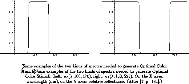
The spectral reflectance is either zero or unity, and in moving through the visible spectrum, there are generally not more than two transitions between these values. Optimal color stimuli are imaginary stimuli in the sense that no actual object surfaces have reflectance curves with abrupt transitions of this kind. However, they are of considerable interest because they represent limiting cases of all (non-fluorescent) object-color stimuli. [] Two types of curves must be distinguished; the first has zero reflectance (or transmittance) at wavelengths and , the second at wavelengths . [Wyszecki \& Stiles 1982][p.181 ff.]

where is wavelength in nm as usual, is the width of the ``gap'' in nm, and is the start of the ``gap'' in nm. Some typical examples of reflectance spectra generated by these functions are shown in Figure .

If we assume a flat-spectrum (white) light source, defined by , the light reaching the sensors has a spectrum identical to the reflectance function, and we can compute Optimal Color Stimulus coordinates for linearly responding sensors as follows:

where is a list of expressions with index variable ranging from 1 to N, N is the number of dimensions (basis functions) of the color space, is the spectral sensitivity of each of the basis functions, and and represent the lower and upper limit of sensitivity for the sensors used, typically in the neighborhood of 300 and 800 for the human visual system, respectively. By varying and over the visible wavelength range, and plotting the resulting points and , we can compute the shape of the OCS surface. It is made up of two ``halves'' that fit together like clam shells, corresponding to the set of points and .

Now we need to choose sets of basis functions . If we choose the standard CIE XYZ functions (Section p. ), we get the result shown in Figure . This is the typical ``torpedo-like shape'' that [Wyszecki \& Stiles 1982] refer to. For the actual computations involved in creating figures ff, I used a computationally more efficient technique than suggested by equations ff, making use of the special properties of the functions and and using a list of partial integrals as a kind of cache.

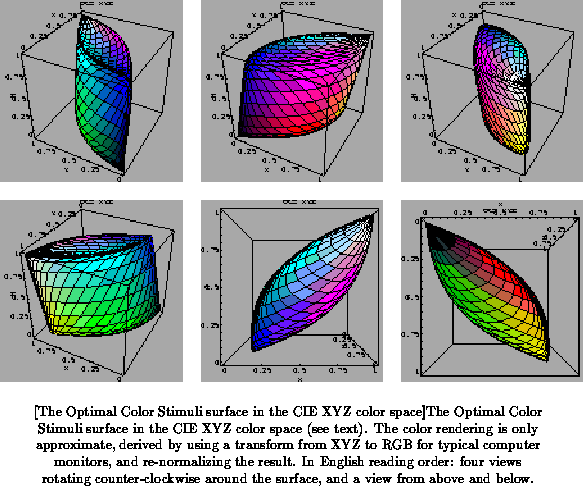
The surface color in Figure is (necessarily) only an approximation, derived as follows:

where are normalized RGB coordinates, is a limiting function serving to limit RGB coordinates to the gamut of the display device, is a linear transform from XYZ to ``typical computer monitor'' RGB coordinates such as the ones given in [Rogers 1985] or [Hill 1990], are the CIE XYZ coordinates computed with equations ff (p. ), and is the set of RGB coordinates corresponding to a maximum radiance flat spectrum (white). The latter is used as a normalization factor for display purposes, which is basically Von Kries adaptation [Wyszecki \& Stiles 1982]. It is clear from these equations that the displayed color has to be approximate, because of the limitations of the gamut of the display device, the ``typical'' transform used, and the inability to control for such things as gamma correction. Nevertheless, the rendered color is a reasonable indication of the ``real'' color corresponding to that particular point on the OCS surface.

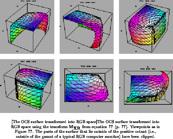
It is interesting to note that only a relatively small volume of the XYZ cube actually corresponds to physically realizable colors. The same is true of course if we compute the OCS surface in RGB coordinates, but the intersection of the volume enclosed by the OCS surface with the all-positive (i.e., displayable) RGB subspace is even smaller than in the XYZ case (Figure ).

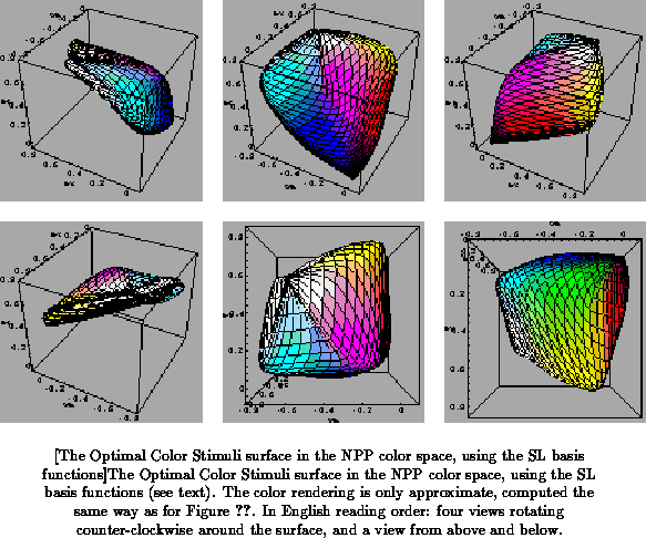
Choosing different basis functions results in different shapes of the OCS surface. The computation for the SL functions is somewhat more involved then for the CIE XYZ functions, because of the nonlinearities. The equations for computing points on the surface are

where symbols are as in equations ff (p. ), being the sigmoid component, and being the linear component of the basis functions. Since the value of the sigmoid function is a non-linear function of its input, there is an issue here with respect to scaling the linear responses that was not relevant for the linear CIE XYZ functions. We have to determine values for the constants . The method I have used is essentially scaling with respect to the equal-energy (EE) or ``white'' response. The argument goes as follows. We want to scale the brightness (Br) dimension to range from perceived black to white, without affecting the adaptive state of the visual system. Once I have determined a scaling factor for the Br dimension I will use it to scale the other dimensions as well. It is justifiable to use the same scaling factor for all color-space dimensions, since the functions I derived in sections ff (p. ff) preserve the ratios of responses among the cell types involved. Assuming (as usual) that the perception of ``white'' arises from the viewing of a stimulus with a flat equal-energy spectrum , we can normalize responses with respect to this type of stimulus. Since ``white'' is at the top of the Br dimension (always within the adaptive range), a flat spectrum ``white'' (maximum relative radiance) stimulus must result in the maximum response for the Br function, which is the function value at the wavelength of maximum response and at maximum relative radiance:

The response of the linear Br function to a flat-spectrum ``white'' stimulus is given by

And the desired scaling factor is then just the quotient of the two:

The normalized response of a linear function to a stimulus is then simply

The final SL normalized function value is

as discussed above. Applying this normalization to the SL functions and computing the OCS surface results in the shape shown in Figure .

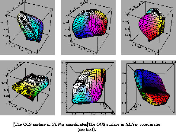
For the SLN functions the normalization process is as described for the SL functions, except the scaling factor is computed using the function, and each of the six response functions is normalized individually before being combined into 3 dimensions. The resulting OCS surface is shown in Figure .

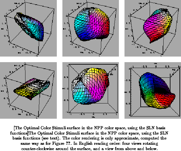
Since the white point is slightly off-center (i.e., not on the axis) in the SLN space as shown above, I will apply a final linear transform to the color-space coordinates to compensate for this. Since the SLN coordinates are in the range (Section p. ), the transform we want is given by

where and are the and coordinates of the white point, respectively. I will refer to the transformed coordinates as the coordinates, and the corresponding color space as the NPP color space. The OCS surface in coordinates is shown in Figure .

The gray axis is now perfectly vertical, the coordinates of black being , and white being . The extrema of the OCS surface coordinates have now changed from to , which makes the complete color stimuli solid fit inside a unit magnitude cube.

For comparative purposes, the OCS surface is represented in CIE L*a*b* coordinates (Figure ), which represents an attempt to create a perceptually equidistant color space for reflected light (Section p. ). The L*a*b* model is based on psychophysical principles only, however, not on neurophysiological data as the NPP space is.

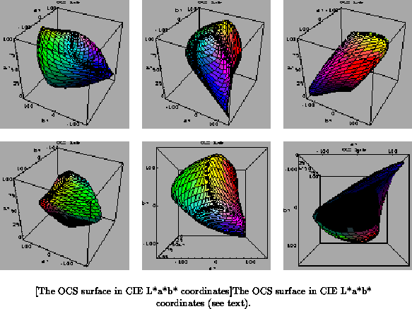
Although the order of hues around the NPP and L*a*b* spaces is the same, there are marked differences in the overall shapes (e.g. the sharp protrusion of the L*a*b* space in the blue region is absent in the NPP space), and the relative positions and areas that certain colors occupy on the respective surfaces. These differences and their implications for theories of color perception remain to be investigated in detail, but that is outside of the scope of this dissertation. In the next section we will look at similarities between the NPP and other spaces to the Munsell system, another often-used psychological color-order system.

In [Wyszecki \& Stiles 1982], only black and white hand-drawn approximations of the OCS shape (in different color spaces, but not NPP of course) are shown, and I am not aware of any attempts to define the complete shape and its surface color analytically as I have done. Later, I will use the OCS surface as a frame of reference to investigate the distribution of basic color categories. It is well suited for that purpose, since it represents the limit of all physically possible surface reflectances (giving rise to color perception when viewed under an appropriate light source), and I can represent it in the neurophysiologically-based NPP space.