Previous: The Normalized Gaussian Category Model Up: From Color Space to Color Names Next: Fitting the Model to the Data

Locating the Berlin and Kay Color Stimuli in the Color Space

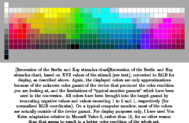
Before we can apply the category model described in the previous section to Berlin and Kay's color naming data, we need to quantify the stimulus set they used for their experiments. As described in Section , they used a set of 329 Munsell color chips consisting of 40 equally spaced hues at 8 equally spaced brightness (Value) levels each, all at maximum saturation (Chroma), and a gray scale consisting of nine equally spaced brightness (Value) steps. They asked subjects to point out both the extent and the foci of the basic color categories of their native language on the array of color chips, viewed under a light source approximating the CIE standard source A (Figure ).

In the following sections I will always use the CIE XYZ space, the CIE L*a*b* space, and the NPP color space for comparative purposes. The XYZ space is in a sense ``the mother of all RGB spaces'', since the various RGB spaces are simple linear transforms of it. It is generally accepted as an approximation to the spectral sensitivities of the human cone photoreceptors, and thus a ``primary'' representation, as close to the sensor as we can hope to get. The L*a*b* space is defined by the CIE to be perceptually equidistant across (most of) the color gamut, and is often used as a reference in color work. It is a non-linear transform of the XYZ space. It also performs very well for our purpose, as shown below. The NPP space is of course the one that we derived from neurophysiological measurements in Chapter , and is also a non-linear transform of the XYZ space. We use this space to attempt to link the category model to the underlying neurophysiology.

The conversion from Munsell coordinates, in which the stimulus set is defined, to CIE XYZ coordinates, which is the basis for the color spaces we are interested in, is non-trivial, and there is no simple mathematical conversion possible. Fortunately, the Munsell set of standard color reference chips, from which the Berlin and Kay set is chosen, has been measured spectrophotometrically and converted to CIE xyY coordinates in the past [Newhall et al. 1943]. After conversion from CIE xyY, we obtain unnormalized CIE XYZ coordinates for each of the stimuli contained in the Berlin and Kay set. To normalize the coordinates to the unit cube, with the gray axis going from to , I used Von Kries adaptation:

where is the vector representing the unnormalized stimulus values, and is the vector representing the unnormalized white reference stimulus values. Although Berlin and Kay's gray axis only runs from Munsell Value 1 to 9, I used the coordinates of Munsell Value 10 as white reference, since that is the maximum Munsell Value defined, i.e. the ``whitest white'' available. Although Von Kries adaptation cannot theoretically be shown to exactly undo all the effects of a non-flat spectrum light source, it works well enough in practice to be allowable, especially with a light source that is as close to a flat spectrum as the CIE C source used in these measurements [Wyszecki \& Stiles 1982]. The obtained stimulus set is shown in Figure , represented in CIE XYZ, CIE L*a*b*, and NPP coordinates.

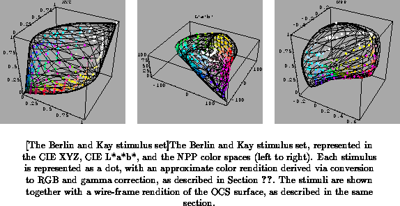
Some interesting things to note about this figure are:

• In all color spaces, the stimuli lie near or on the OCS surface, as is expected since they represent the maximum saturation levels available at each brightness and hue value. The OCS surface was computed entirely independently, however, as described in Section . This provides a nice cross-check for the consistency of both data sets.

• The spacing of the stimuli varies in the various color spaces. Although it is difficult to see from the figure, the spacing is most equal in the CIE L*a*b* space, which was created explicitly for this purpose. The NPP space is less than perfect in this respect. One might speculate that this is due in part to the relatively early stage in the visual neural pathway from which the corresponding measurements are collected, and that perceptually equal spacing is an effect of subsequent transformations of the neural signals.

• There are some irregularities in the spacing of the stimuli, particularly in the blue region. These irregularities had already been noticed by [Newhall et al. 1943], who contribute them to problems with the underlying CIE standard observer functions themselves. They are not serious enough to cast doubt on the validity of Berlin and Kay's results, however.

In particular, note the irregularities in the lower blue region. I have added Munsell Values 0 and 10 to the gray axis, for a total of 11 stimuli.

Combining the information from Figure with the derived color space coordinates of the stimuli, we can now describe the boundary of a Basic Color category as a polygon passing through the coordinates of each of the boundary stimuli, and the focus of a Basic Color category as the center of mass of the points indicated as focal points. Figure shows the boundaries and foci obtained in this way.

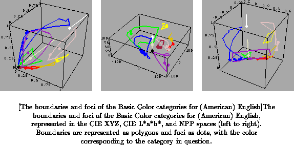
Note that the shape and size of the polygons is different in different color spaces, and that in general a straight line on the Berlin and Kay chart does not necessarily translate into a straight line in the color space, since the stimuli are lying on or near a curved surface.